In today’s data-driven world, it is crucial to make quick decisions based on accurate information. But what if your data is not as fresh as you think?
This blog post dives into the concept of data timeliness, with a specific focus on ingestion delay. We will explore how to monitor this delay using the DQOps platform to ensure you are working with the latest information, ultimately empowering you to make better business decisions.
Table of Contents
What is data timeliness?
Timeliness refers to the expected availability and accessibility of data within a reasonable timeframe. It reflects how quickly data is captured, processed, and made available for analysis. Timely data is crucial for making informed decisions based on the latest information.
We can only measure timeliness for datasets containing business events with timestamp columns. These columns capture the specific point in time when a business event occurred. For example, Sales facts would have a sales_date column, Business transactions would have a transaction_timestamp, Logs would have a timestamp for when the log entry was generated, and Clickstreams would have an impression_timestamp for when the ad impression occurred. We will refer to this column as the event_timestamp throughout this article.
Many target tables loaded through ETL processes also have an inserted_at column. When the data record is loaded, this column is automatically populated with the current timestamp. The specific name may vary depending on your data platform’s naming conventions. The simplest way to populate inserted_at during data loading is to configure it as a default value that calls the database engine’s function to capture the current system time.
With both event_timestamp and inserted_at columns in your monitored table, we can now explore how to measure timeliness. There are three types of data timeliness measures: data freshness, data staleness, and ingestion delay.
Data freshness is the age of the most recent row in the monitored table. We calculate it by finding the difference between the most recent event timestamp in the table and the current system time at the time of observing the freshness.
Data staleness measures the time since the target table was recently loaded.
Ingestion delay measures the time it takes for the data pipeline or the ETL process to pick up the most recent data and load it into the target table.
You can read more about the types of data timeliness checks mentioned above in a separate blog post. The following time diagram compares all timeliness metrics supported by the DQOps platform.

What is ingestion delay?
Ingestion delay refers to the time it takes for your data pipeline to process and load a record after the corresponding business event occurs. In simpler terms, it is the lag between when something happens (e.g., a sale) and when that information is reflected in your data warehouse. This delay can occur during data processing itself or between scheduled pipeline runs.
To measure ingestion delay, we look at two timestamps associated with each data record:
- Event timestamp (event_timestamp): This captures the specific time the business event happened. For instance, it might reflect when a customer places an order or signs up.
- Loading timestamp (inserted_at): This indicates when the record was successfully loaded into your target data warehouse table.
We can calculate the time it took to process and load the data using the following formula:
MAX(inserted_at) – MAX(event_timestamp)
Important Considerations
- Data Reloads: Ingestion delay can be sensitive to full reloads of your data warehouse. When existing rows are deleted and reloaded, their loading timestamps change. This might temporarily create the impression of a slower pipeline than usual.
- Long Delays vs. Reloads: A long ingestion delay doesn’t necessarily signify a problem. It could simply indicate a recent data reload, which is a standard operation.
- Date-Partitioned Data: For tables partitioned by date (e.g., daily or monthly partitions), ingestion delay becomes even more critical. DQOps offers partition checks that calculate the delay for each partition, allowing you to monitor when specific date ranges were loaded or reloaded. This helps ensure your most recent data is readily available for analysis.
Strategies for minimizing ingestion delay
There are several ways to minimize ingestion delay and ensure your data is as timely as possible:
- Real-Time Data Pipelines: Utilize technologies like Apache Kafka or Apache Flink to capture and process data as it’s generated, minimizing the lag between data creation and availability.
- Stream Processing: Implement stream processing frameworks to analyze data in real time, allowing you to react quickly to changes and identify emerging patterns.
- Optimize Data Architecture: Evaluate your data architecture and identify bottlenecks that slow down data ingestion. This might involve scaling resources or optimizing data transformation processes.
- Monitor and Alert: Continuously monitor ingestion delays and set up alerts to notify you when data pipelines encounter issues. This allows for prompt intervention and troubleshooting. To monitor data timeliness you can use the DQOps data quality platform.
Data quality best practices - a step-by-step guide to improve data quality
- Learn the best practices in starting and scaling data quality
- Learn how to find and manage data quality issues
Measuring ingestion delay with the DQOps platform
To measure the delay in data ingestion, you can use the data_ingestion_delay check within the DQOps platform. DQOps supports configuring data timeliness monitoring checks both in a YAML file and using a user interface.
Identifying and configuring event and ingestion timestamp columns
Before activating the data_ingestion_delay data quality check in the DQOps platform, you must enter an additional configuration for the monitored table. DQOps must know which columns in the table store event timestamp and which loading timestamp (ingestion timestamp) values.
You have to configure both of the column names:
- The event_timestamp_column parameter stores the name of the column containing the most recent business action.
- The ingestion_timestamp_column parameter stores the name of the column containing the timestamp when the row was loaded into the target table.
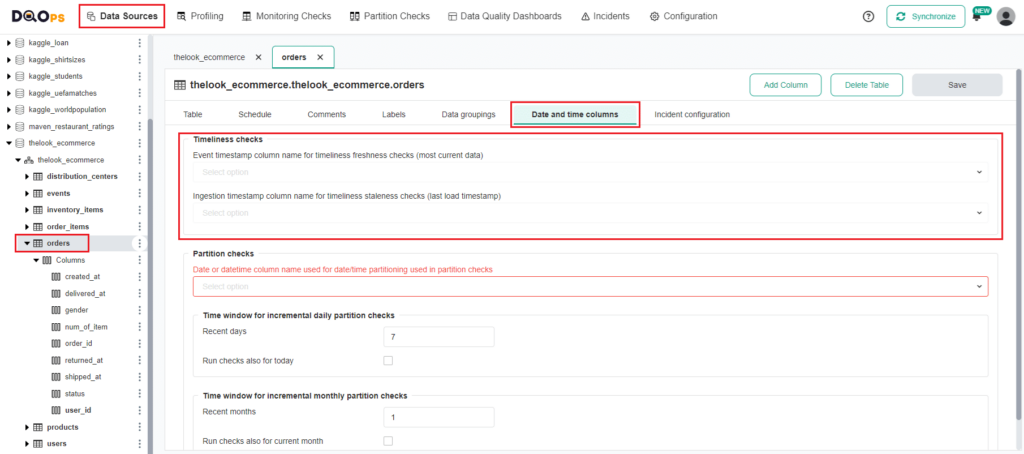
To configure the columns using the user interface:
- Go to the Data Source section and select the table of interest from the tree view on the left.
- Click on the Date and time Columns tab.
- From the dropdown menu, select the column names for the event timestamp and ingestion timestamp.
- Click the Save button located in the top-right corner.
Configuring data_ingestion_delay data quality check in the YAML file
You can configure the data_ingestion_delay check in the YAML file or using the user interface.
The example below shows how to configure the ingestion delay check in a YAML file. It contains the column names of the event and ingestion timestamps. The name of the monitored table is not shown in the YAML file because DQOps follows the principle of “configuration by convention,” storing the table name as the file name.
The check configuration also includes a threshold parameter max_days, which determines the length of an ingestion delay that should trigger a data quality issue at en error severity level.
					apiVersion: dqo/v1
kind: table
spec:
  timestamp_columns:
    event_timestamp_column: event_timestamp
    ingestion_timestamp_column: inserted_at
  monitoring_checks:
    daily:
      timeliness:
        daily_data_ingestion_delay:
          error:
            max_days: 2.0
Running data_ingestion_delay data quality check
In the DQOps platform, you can run checks using either the user interface or the Shell. To run the data_ingestion_delay check from the user interface, simply navigate to the Monitoring checks section and select the table of interest.
Refer to our documentation to learn how to add a new connection and import tables.
Select the table of interest. This will display a check editor in the main workspace. The data_ingestion_delay check is within the Timeliness group categorized as an advanced check. To display advanced checks, click on the Show advanced checks checkbox.
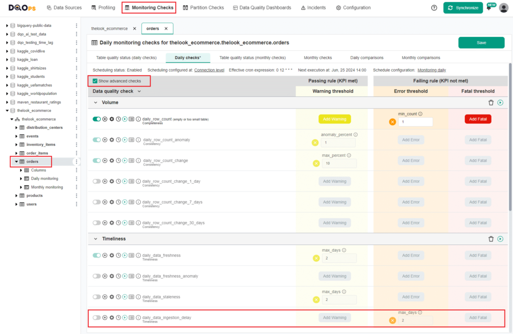
To activate the check, toggle the enable switch. Next, set the maximum number of days as an accepted value or leave it as the default, which is 2 days. If the result of the check is less than the maximum number of days, an alert will be triggered. Finally, run the check by clicking the green Run button.
For a complete guide on how to run checks, refer to DQOps documentation.
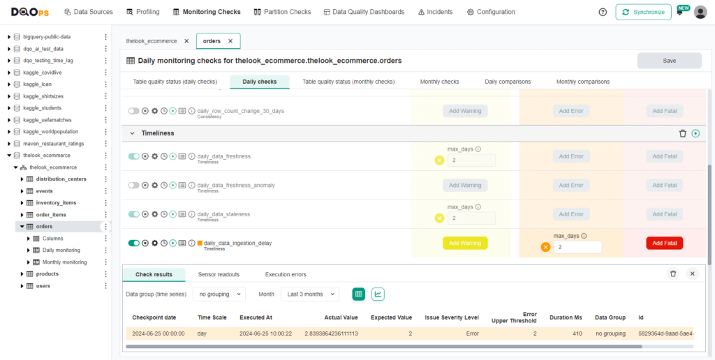
The check resulted in an Error, as indicated by the orange square next to the check name. You can view the results by hovering over the orange square or accessing more detailed results by clicking on the Results icon. In our case, the ingestion delay was 2.8 days, exceeding the maximum accepted value of 2 days.
Reviewing results on the dashboards
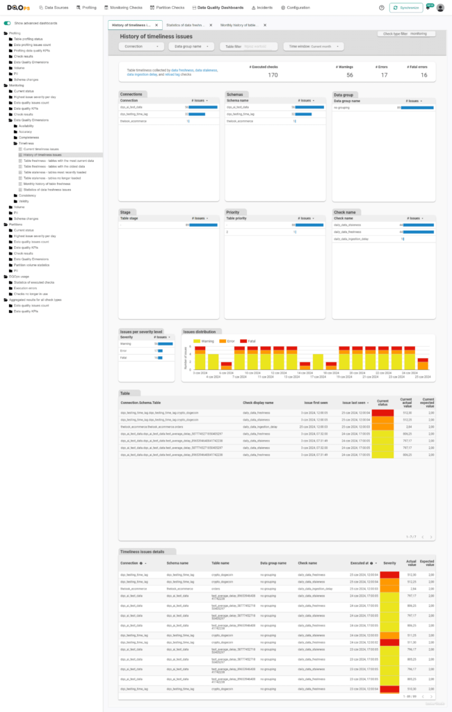
The DQOps platform includes multiple built-in data quality dashboards specifically dedicated to data timeliness. These dashboards enable users to track and review various timeliness issues from different perspectives. The documentation provides details about the different timeliness dashboards.
Below is an example of an advanced dashboard showing the History of timeliness issues, which allows for a review of the reliability of the timeliness dimension for tables.
Summary
Stale data can cause a cascade of problems, leading to outdated insights, missed opportunities, and poor decision-making. The DQOps platform enables you to monitor data ingestion delays and receive notifications about any issues. By minimizing data ingestion delays, you can make more informed, data-driven decisions based on the most up-to-date information.